Off-Policy RL for LLMs, Explained Visually

Part 1 derived the policy gradient for language models.⊕ A cartoon of on-policy training. The sampler is the trainer, so training heads straight for high reward. It ended by describing the on-policy assumption, which says that the model generating the completions is the exact one we differentiate during training. That assumption rarely holds in practice. This post covers what happens when training goes off-policy and the two main ways to correct for it, importance sampling and score centering.

Recap

Part 1 ended by looking at the policy gradient one token at a time. At a given position in the completion, each possible next token $v$ has a probability $p_v$ and a score $s_v = \nabla_\theta \log p_v$. The sampled token $y_t$ contributes $R \, s_{y_t}$ to the policy gradient, where $R$ is the completion’s reward.

The key fact from part 1 is that the score has zero mean when the token is sampled from $p$:

$$\mathbb{E}_{y_t \sim p}[s_{y_t}] = \sum_v p_v \, \nabla_\theta \log p_v = \nabla_\theta \sum_v p_v = 0$$

The same fact is why subtracting a baseline $b$ from the reward doesn’t change the expected gradient, since $b \, s_{y_t}$ averages to zero as well. Off-policy, the score no longer averages to zero, so both properties break.

The examples in this post reuse the prompt from part 1, “What is 17 × 24?”.⊕ The running example from part 1. After “17 × 24 = 17 × 20 + 17 × 4 = 340 +”, the model gives the correct next token, 68, a probability of 0.82, and the slip 58 a probability of 0.07. Choosing 68 leads to the right answer (408) and reward 1, while the slip 58 leads to a wrong answer and reward 0.

Where off-policy data comes from

Training is off-policy whenever the completions come from a distribution $q$ other than the policy $p_\theta$ being updated. In LLM RL, an inference engine generates the rollouts and a training framework updates the weights, so we’ll call $q$ the sampler and $p_\theta$ the trainer. Any gap between the two is called the training-inference mismatch. It is famously hard to get rid of, and it can quietly degrade training or collapse the reward entirely.Supervised fine-tuning, by contrast, happily trains on text generated by an entirely different model or written by a person, with no correction at all.

There are three common causes of unwanted mismatch. Two come from timing, because the sampler generated the rollouts using older weights than the trainer’s current ones. The third comes from computation, because the two engines compute slightly different probabilities even from the same weights.

Multiple updates per batch

Generating rollouts is often the most expensive part of RL for LLMs, so trainers usually split each batch of rollouts into minibatches and take one gradient step on each. DAPO, for example, splits each batch into 16 steps. Only the first step is on-policy. After that first step, $\theta$ has moved, and every later minibatch comes from a slightly older policy.Classic PPO goes further and makes several passes, or epochs, over the same batch. Recent LLM recipes mostly avoid this for stability. TRL’s GRPO trainer, for example, defaults to a single pass. This staleness is a deliberate tradeoff for sample efficiency, and proximal policy optimization (PPO) introduced ratio clipping specifically to handle it.

Stale weights

To keep GPUs busy, large-scale RL runs inference and training asynchronously and serves rollouts with continuous batching. While the sampler is still generating a slow rollout, the trainer keeps updating the weights on faster ones that already finished. By the time that rollout completes, the trainer has moved on to a newer checkpoint, and if new weights sync mid-generation, a single rollout can even span several checkpoints. This staleness is worst in long agentic tasks, where some episodes finish in minutes and others take hours or days.

Numerical differences

Even with fresh weights and a single gradient step, the sampler and trainer rarely compute the exact same probabilities. They are usually different programs: after the sampler generates a rollout, the trainer runs its own forward pass over those tokens to compute log-probabilities for the policy gradient loss. Even on identical weights, the two forward passes can disagree for two reasons:

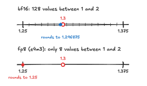
• Different precisions and codebases. The two engines may run at different precisions, such as an fp8 or int8 sampler paired with a bf16 trainer, or a quantized KV cache.A floating-point format can store only a fixed number of values between consecutive powers of two, and every weight and activation is rounded to the nearest one. bf16 has 128 values between 1 and 2, spaced $1/128$ apart, while fp8’s e4m3 format has only 8, spaced $1/8$ apart. So the same weight, 1.3, is stored as 1.296875 in bf16 but 1.25 in fp8. They may also come from independent codebases, each with its own hard-to-detect bugs.
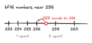
• Same kernels, different shapes. Even with identical, correct kernels, the sampler decodes one token at a time while the trainer scores the whole completion in one forward pass. Different input shapes can change the order of floating-point reductions, and floating-point addition isn’t associative.Addition is associative when $(a + b) + c$ always equals $a + (b + c)$. Floating-point addition isn’t, because each intermediate sum is rounded to the nearest representable number, and representable numbers get sparser as they grow. In bf16, they are 1 apart just below 256 but 2 apart above it, so 257 has no exact representation and rounds back to 256. So $(1 + 1) + 256 = 258$, but $1 + (1 + 256)$ rounds to $256$ at each step. When different kernels add a long sum of logits or attention scores in a different order, the final result can differ slightly for the same reason. Batch-invariant kernels remove the dependence on shape, but they take real engineering effort and cost GPU utilization. Running both engines in fp16 instead of bf16 greatly reduces the mismatch, but doesn’t eliminate it.

At the “340 +” slot from part 1, for example, the two engines can disagree slightly about the next token, even with identical weights:

Here the trainer gives the slip 58 a probability of 0.07, while the sampler used 0.06. Small discrepancies like this show up at every token of every rollout.

Small as they are, these differences can build up over training and grow larger in long responses, where the reward signal is already thin (a fixed number of bits of feedback spread across more tokens) and asynchronous execution adds staleness on top.

All three sources of mismatch come from deliberate throughput tradeoffs. Multiple updates per batch, asynchronous rollouts, and fast inference kernels make RL practical at scale, and giving them up would make training much slower. So the practical question is how to train well on off-policy data.

Sampling from a better model

In all three cases above, the sampler is meant to be a copy of the trainer, so any gap between them is error. Other times, the data comes from a different source on purpose, because it can show the trainer something it wouldn’t produce on its own:

• A stronger model. Rollouts from a larger or better model can show the trainer solutions it would rarely find on its own. LUFFY, for example, mixes reasoning traces from a stronger model into on-policy RL.
• A teacher with extra context. Even the same model can act as a teacher if its prompt includes the reference solution or other privileged information; the student then learns from those completions without seeing the hint. STaR’s rationalization step works this way, giving the correct answer as a hint. Instead of generating completions, the teacher can also score the student’s rollouts.
• People. Hand-written demonstrations are the oldest kind of off-policy data, and SFT trains on them with no correction at all.

Here the gap between sampler and trainer carries useful signal rather than error, and the question is how much of it the trainer should absorb. The gap can also be large, which weakens corrections that assume a small mismatch. The rest of this post focuses on unwanted mismatch.

Why off-policy updates go wrong

The policy gradient is an expectation over completions from the policy being trained. With off-policy data, the REINFORCE estimator averages the same quantity over the sampler’s completions instead. The trainer computes the same formula on each completion, $R(y) \, \nabla_\theta \log p_\theta(y)$, but averaging it over $q$ instead of $p_\theta$ changes the expectation:

$$\begin{aligned} &\mathbb{E}_{y \sim q}\big[R(y) \, \nabla_\theta \log p_\theta(y)\big] \\ &\quad \neq \mathbb{E}_{y \sim p_\theta}\big[R(y) \, \nabla_\theta \log p_\theta(y)\big] = \nabla_\theta J(\theta) \end{aligned}$$

To see what goes wrong, look at a single token position under a constant reward.

A thought experiment: constant reward

Suppose every completion earns the same reward, $R = 1$, no matter what it says.⊕ There is nothing to learn, and on-policy the expected update is exactly zero. At each position, the sampled token’s score averages to $\mathbb{E}_p[s_{y_t}] = 0$, so $\mathbb{E}_p[R \, s_{y_t}] = R \cdot 0$.

Off-policy, the sampler $q$ draws the token, while the trainer $p$ still computes its score. The average score is then

$$\bar{s} = \mathbb{E}_{y_t \sim q}[s_{y_t}] = \sum_v q_v \, \nabla_\theta \log p_v ,$$

and the zero-mean identity no longer applies, because the weights $q_v$ are not the probabilities $p_v$ inside the score. In general $\bar{s} \neq 0$, so the expected update $\mathbb{E}_q[R \, s_{y_t}] = R \, \bar{s}$ isn’t zero either. The model moves even though the reward carries no information.

That update points along $\bar{s}$, which is the negative gradient of the cross-entropy loss $-\sum_v q_v \log p_v$ between $q$ and $p$. Minimizing that loss trains $p$ to imitate $q$, so with a constant reward, off-policy policy gradient is supervised distillation of the trainer toward the sampler. It pulls $p$ toward whatever $q$ does, including every quirk of its numerics or staleness.

Drift and signal

When the reward varies across completions, the covariance identity $\mathbb{E}[AB] = \mathbb{E}[A]\,\mathbb{E}[B] + \mathrm{Cov}(A, B)$ splits the update into a part from the mismatch and a part from the reward. As before, fix the prompt and the prefix before position $t$. Averaging over the next token $y_t \sim q$ and the rest of the completion (which determines $R$) gives:

$$\underbrace{\mathbb{E}_q[R \, s_{y_t}]}_{\text{policy gradient update}} = \underbrace{\mathbb{E}_q[R] \; \bar{s}}_{\text{drift}} + \underbrace{\mathrm{Cov}_q(R, \; s_{y_t})}_{\text{signal}}$$

• The signal term is the only one that depends on which tokens led to which rewards. It is large when tokens that tend to produce high reward have scores pointing in a consistent direction. This is the part of the update we actually want.
• The drift term depends on the rewards only through their average. Its direction is $\bar{s}$, the distillation direction from the thought experiment, scaled by how much reward the prefix typically earns.

On-policy, $q = p$, so $\bar{s} = 0$ and the drift term vanishes. It exists only because of the mismatch.

Why drift compounds

Distilling toward a sampler that never changes is benign.⊕ A frozen sampler: training settles short of the peak. Its target stays put, so $p$ simply converges toward $q$ and stops. But in RL for language models, the sampler doesn’t stay fixed. Every weight sync refreshes it from the trainer’s latest weights, and it then adds its own numerical bias on top. So the sampler is a slightly biased copy of the trainer that moves whenever the trainer does.

That closes a feedback loop.⊕ A synced sampler: the reward peaks, then falls. Each step pulls the trainer toward the biased sampler, and the next sync copies those new weights back into the sampler, which applies its bias again. If that bias points the same way from one step to the next, each pull adds to the last and the error keeps growing. A quantized sampler could produce this kind of persistent bias: its rounding error is a deterministic function of the weights, and the weights change only a little per step (though nothing guarantees that successive pulls line up).We don’t yet know whether real numerical bias persists across steps. The trainer–sampler gap has been seen to grow during training, but kernel errors also look like symmetric noise, which would partly cancel. That may explain why off-policy runs often look fine for a while and then suddenly collapse.

At scale, Modal saw this pattern training a 35B model on agentic coding. In every run that collapsed, the sampler–trainer KL had first grown threefold or more. Samplers matched to the trainer’s hardware and precision started with about a quarter of the mismatch, but GRPO still collapsed on them, just later. With the corrections below, runs stayed stable at nearly five times the mismatch. So the mismatch’s growth predicted collapse, and its starting size didn’t.

Evidence: frozen vs synced samplers

This feedback loop makes a testable prediction. With a frozen sampler, training with $+1/0$ rewards is ordinary SFT on the correct completions, which is stable even on text from a completely different model. With a synced sampler, the same rewards should become unstable, because the sampler is a biased copy of the trainer that keeps getting refreshed.

Marek and Ryabinin test this by training Qwen3-1.7B on the Countdown arithmetic game, with the sampler’s weights slightly perturbed to create a controlled mismatch. They compare three reward schemes, $+1/0$, $+1/{-}1$, and group-centered, with the sampler either frozen (never updated) or synced from the trainer after every step.⊕Redrawn from Marek and Ryabinin (2026), Figure 2. Each curve is the mean of three seeds.

• With a frozen sampler, only $+1/0$ is stable, since it reduces to SFT on the correct completions. The two schemes with negative rewards collapse within 20 steps for a different reason: pushing down the probability of fixed bad completions has no floor, as $\log p$ can fall to $-\infty$.
• With a synced sampler, the ordering flips. $+1/0$, the SFT-like setting, collapses first, $+1/{-}1$ lasts longer, and group-centered rewards stay stable.

The drift term explains the ordering with a synced sampler. Its size is set by the average reward $\mathbb{E}[R]$, and at the same accuracy, the three schemes give very different averages:

• With $+1/0$ rewards, $\mathbb{E}[R]$ equals the accuracy, about 0.5 to 0.6 in these runs, so the drift is large from the first step. This run collapses first.
• With $+1/{-}1$ rewards, $\mathbb{E}[R] = 2 \cdot \text{accuracy} - 1$. At the starting accuracy of about 45%, that’s close to zero, and it reaches only about 0.4 once the model improves. The drift is smaller, and this run lasts longer before collapsing.
• With group-centered rewards, $\mathbb{E}[R]$ is zero at the prompt by construction, whatever the accuracy.This holds when every completion counts equally, as in the original GRPO loss, which averages over each completion’s tokens. Variants like DAPO and Dr. GRPO weight every token equally instead, so longer completions count more. The drift shared by every token then scales with a length-weighted average advantage, $\sum_i A_i L_i / \sum_i L_i$ for completions of length $L_i$, which is zero only if right and wrong completions are equally long. This run stays stable.

Even when $\mathbb{E}[R]$ is zero across whole completions, though, it rarely stays zero at individual prefixes.

Drift survives group centering

Group centering, as in GRPO, works at the sequence level. It subtracts the group’s average reward from each completion’s reward, and every token in the completion shares that same advantage. Because those advantages average to zero across the group, you might expect the drift to vanish. At any token position, though, drift scales with the expected advantage at that prefix. That token-level average can be far from zero even when the whole group averages to zero.

A prefix that has already made the “340 + 58” slip is headed for a wrong answer, so its expected advantage is negative. A prefix that is on track, like “340 + 68”, has a positive one. These prefix-level averages are largest in magnitude where the outcome is already mostly decided. There the later tokens barely affect the reward, so the signal is near zero and the update is almost pure drift.

Group centering shrinks the drift, which explains why it is the most stable of the three schemes above, but it doesn’t eliminate it. Promising prefixes still pull the trainer toward the sampler, and mistakes push it away, even at tokens that don’t affect the reward.

Importance sampling

The classical fix for training on samples from the wrong distribution is importance sampling, a general Monte Carlo technique for estimating an expectation under one distribution using samples drawn from another.⊕Here we use only the reweighting step, which some authors call importance weighting. Classic importance sampling also chooses the distribution to sample from, often to reduce variance. In RL the samples come from whatever sampler produced them, so there is no such choice to make. The RL literature still calls it importance sampling, and method names like TIS and MIS follow that usage.

Reweighting the samples

For any function $f$,⊕ Weighted by the exact importance ratios, the sampler’s bias no longer matters. The trainer follows the on-policy path.

$$\begin{aligned} \mathbb{E}_{y \sim p}[f(y)] &= \sum_y p(y) \, f(y) \\ &= \sum_y q(y) \, \frac{p(y)}{q(y)} \, f(y) \\ &= \mathbb{E}_{y \sim q}\Big[\frac{p(y)}{q(y)} \, f(y)\Big] \end{aligned}$$

Each sample is weighted by its importance ratio $p(y)/q(y)$. If the sampler generates a completion more often than the trainer would, the completion gets down-weighted, and if it generates one less often, that one gets up-weighted. On average, the samples then count as if they had been drawn from $p$. The only requirement is that the sampler can generate everything the trainer can: $q(y) > 0$ wherever $p(y) > 0$.Top-p and top-k sampling break this, because tokens outside the nucleus have $q = 0$ but $p > 0$. The usual fix, used by MAI-Thinking-1 and DeepSeek, is to apply the sampler’s mask in the trainer too, so $p$ has the same support as $q$.

Applied to the policy gradient, with $f(y) = R(y) \, \nabla_\theta \log p_\theta(y)$, this gives an unbiased estimate from the sampler’s rollouts:

$$\nabla_\theta J(\theta) = \mathbb{E}_{y \sim q}\big[\underbrace{\tfrac{p_\theta(y)}{q(y)}}_{\text{importance ratio}} R(y)\nabla_\theta \log p_\theta(y)\big]$$

Reweighting is also cheap. The trainer already computes $p_\theta(y)$ in its forward pass, and inference engines can return the log-probabilities of the tokens they sample at almost no extra cost.

Why sequence-level ratios explode

A completion’s probability is the product of its token probabilities, so its importance ratio is a product of per-token ratios:

$$\frac{p_\theta(y)}{q(y)} = \prod_{t=1}^{T} \underbrace{\frac{p_\theta(y_t \mid y_{<t})}{q(y_t \mid y_{<t})}}_{r_t}$$

Each factor is usually close to 1,⊕In the worked example from earlier, at “340 +” in 17 × 24, the trainer gives the slip 58 a probability of 0.07 and the sampler 0.06, so its factor is $0.07 / 0.06 \approx 1.17$. The factor for 68 is $0.82 / 0.83 \approx 0.99$. but a completion has hundreds or thousands of them, and small factors compound. A per-token ratio of 1.01, repeated over 1,000 tokens, compounds to $1.01^{1000} \approx 21{,}000$, and 0.99 shrinks to $0.99^{1000} \approx 0.00004$.

Real per-token ratios aren’t constant. They wander above and below 1, but under the sampler each one averages to exactly 1, $\mathbb{E}_q[p_v / q_v] = \sum_v p_v = 1$, which is what keeps importance sampling unbiased. The log of the sequence ratio is a sum of these small random terms, so it behaves like a random walk whose spread grows with the square root of the length. A simulation with small random per-token ratios shows how quickly the rollouts’ weights spread apart:⊕Each token’s log-ratio is drawn from a normal distribution with mean −0.05²/2 and standard deviation 0.05, so a typical ratio is within about 5% of 1, and the ratios average exactly 1. The y-axis uses a log scale, where each path is a random walk that drifts downward, so most rollouts end well below 1. The few that end above it hold the mean at 1. Each rollout’s gradient is multiplied by its weight, so the ×8.5 rollout counts about 300 times as much as the ×0.03 one, but nothing about it is more informative. Its tokens’ small disagreements just happened to line up. The histogram shows where 5,000 rollouts end. The shares in the text use 20,000, and the effective sample sizes split those into batches of 512.

The weights still average to 1, so the estimate stays unbiased, but that average is shared very unevenly. In this simulation, most rollouts get a weight below 1Each token’s ratio averages to exactly 1 under the sampler, $\mathbb{E}_q[r] = \sum_v q_v \, p_v / q_v = 1$, but its log does not average to 0. Because log is concave, $\mathbb{E}_q[\log r] \le \log \mathbb{E}_q[r] = 0$, and the gap is exactly $\mathrm{KL}(q \,\|\, p)$. So the log of the sequence weight is a random walk that drifts downward, by about $\mathrm{KL}$ per token, while its spread grows only with the square root of the length. Over many tokens, most weights sink below 1, and a few large ones make up the difference. In this simulation, 78% end up below 1, and the share approaches 100% as completions get longer. and barely move the gradient, while a few get large weights and dominate it. As completions get longer, an even larger share falls below 1. At 1,000 tokens, a batch of 512 rollouts weighted this way has an effective sample size of only about 70:This is the effective sample size, $(\sum_i w_i)^2 / \sum_i w_i^2$ for weights $w_i$. It equals the batch size when all weights are equal and approaches 1 when a single weight dominates. It measures how concentrated the weights are. Because the gradient’s noise also depends on the rewards and scores, ESS does not measure that noise directly. The values here are medians over simulated batches of 512. you pay to generate 512 rollouts, but the batch behaves like 70. At 2,000 tokens, it drops to about 20.

Token-level ratios

Sequence-level importance sampling weights every token’s score in a completion by the same number, the product of all its per-token ratios. In practice, almost every method uses token-level ratios instead, weighting each token’s score by its own ratio $r_t$:

$$\sum_t r_t \, R \, s_{y_t}, \qquad r_t = \frac{p_\theta(y_t \mid y_{<t})}{q(y_t \mid y_{<t})}$$

Compared with the exact sequence ratio, this keeps one factor of the product and sets all the others to 1. Every token gets its own correction, but each term reweights only the choice of that token itself. It leaves the prefix before the token and the continuation after it (which decides the reward) uncorrected:

The token itself is corrected exactly. With its prefix held fixed, weighting the sampled token by $r_t$ turns an average over the sampler’s next-token distribution into an average over the trainer’s. In particular, it restores the zero-mean identity from the recap:

$$\mathbb{E}_{y_t \sim q}[r_t \, s_{y_t}] = \sum_v q_v \, \frac{p_v}{q_v} \, s_v = \sum_v p_v \, s_v = 0$$

So the drift term vanishes at every prefix, and only the signal is left.

The prefix and continuation in that term are not corrected. Both still come from the sampler, which decides what prefixes the token is trained on (like “340 +”) and how the completion finishes from there to earn its reward. Correcting for those would require multiplying in the ratios of every other token, which is the product that explodes. So token-level importance sampling is an approximation. It works well when the sampler and trainer are close, since they then reach similar prefixes and finish them in similar ways.

Token ratios are much better behaved than their product, but they are still unbounded. The largest ones come from tokens that the trainer finds much more likely than the sampler did. A token with $q = 0.001$ and $p = 0.01$ gets a weight of 10. Any one such token is rare, but a batch has millions of tokens, so some appear in every batch. A handful of heavily weighted tokens can then dominate the gradient. The weight never divides by zero, since the sampler produced each token and so gave it $q > 0$, but it has no ceiling.

A gradient dominated by a few tokens causes three problems. It points wherever their scores point, so it swings from batch to batch depending on which rare tokens happened to be drawn. The two engines also disagree most on those tokens, often because of numerical error, so the gradient leans hardest on its least reliable parts. And a single huge weight inflates the gradient’s norm. If gradients are clipped by norm, as they usually are, the whole update shrinks, and every other token’s contribution with it.

Bounding the ratio: TIS, MIS, and PPO

So practical methods bound the ratio. They differ in what they do with a token whose ratio falls outside the bounds:

• Truncated importance sampling (TIS) caps the weight at $w_t = \min(r_t, C)$, with $C = 2$ a common default. Tokens with large ratios still count, just by no more than $C$. CISPO caps the weight the same way.
• Masked importance sampling (MIS), introduced as IcePop, keeps $r_t$ inside a band such as $[0.5, 5]$ and drops the token outside it. The idea is that when the two engines disagree that much, the token’s gradient is too unreliable to use.
• Proximal policy optimization (PPO) clips the objective with $\min\big(r_t A_t, \ \mathrm{clip}(r_t, 1 - \epsilon, 1 + \epsilon) \, A_t\big)$, typically with $\epsilon = 0.2$. Taking the minimum of the clipped and unclipped terms makes the objective pessimistic: clipping can only lower it, never raise it. For the gradient, that acts as a one-sided mask. The clip binds only after the advantage has pushed the ratio past the band, above $1 + \epsilon$ for a positive advantage or below $1 - \epsilon$ for a negative one, where the objective flattens and the token’s gradient becomes zero. On the other side of the band, the unclipped term is smaller and the token keeps its full weight $r_t$. For a negative advantage, that leaves every ratio above $1 + \epsilon$ unclipped, so the weight is still unbounded there. DAPO raises the upper edge to 1.28.PPO was designed for multiple updates per batch, where the ratio measures how far the policy has moved since the rollouts were generated. Many implementations compute the denominator by running the old policy in the trainer rather than using the sampler’s logged probabilities, so the ratio never sees the numerical mismatch. IcePop uses both: MIS between sampler and trainer, and PPO clipping between policy versions.
• Group sequence policy optimization (GSPO) stays at the sequence level but replaces the product with the geometric mean of the token ratios, $(p_\theta(y) / q(y))^{1/T}$, and clips that to a very narrow band. Averaging the log-ratios instead of summing them keeps the weight from growing or shrinking exponentially with length.

What bounding the ratio costs

Every bound trades variance for bias.⊕With a fixed cap, like TIS’s 2, this bias doesn’t shrink with more samples. It would if the cap grew like $\sqrt{n}$ in the number of samples $n$ (Ionides, 2008). The ratio was there to remove the drift, and bounding brings some of it back. The zero-mean calculation above shows where it comes from. For weights that depend only on the token, such as TIS’s cap and MIS’s mask, replace $r_v$ with the bounded weight $w_v$.PPO’s clip doesn’t fit this form, because the active side of the band depends on the sign of the advantage (how the whole completion turned out) rather than on the token alone. It still leaves drift behind, just with a messier formula. The expected weighted score at a prefix is then

$$\begin{aligned} \mathbb{E}_q[w_{y_t} \, s_{y_t}] &= \sum_v q_v \, w_v \, s_v \\ &= \sum_v q_v \, w_v \, s_v - \underbrace{\sum_v p_v \, s_v}_{=\,0} \\ &= -\sum_v \big(p_v - q_v \, w_v\big) \, s_v \\ &= -\sum_{v \in \mathcal{B}} \underbrace{\big(p_v - q_v \, r_v\big)}_{=\,0} \, s_v - \sum_{v \notin \mathcal{B}} \big(p_v - q_v \, w_v\big) \, s_v \\ &= -\sum_{v \notin \mathcal{B}} \big(p_v - q_v \, w_v\big) \, s_v , \end{aligned}$$

where $\mathcal{B}$ is the set of tokens whose ratio falls inside the bounds.⊕ TIS: some drift survives, so training settles just off the peak. Those keep $w_v = r_v$, so $q_v \, w_v = p_v$ and they drop out. Drift comes back only through the tokens outside $\mathcal{B}$: when MIS drops a token, it leaves $-p_v \, s_v$ (as if the sampler could never have produced it), and when TIS caps a token at 2, it leaves $-(p_v - 2 \, q_v) \, s_v$.

Bounding caps or drops only tokens whose ratio is far from 1, so it removes drift where the two engines roughly agree and leaves it where they disagree most. A more severe mismatch pushes more tokens outside the bounds and can leave more drift behind.

Score centering

Importance sampling removes drift by reweighting samples, but its practical, bounded versions let some of the drift back in.⊕ Score centering: no drift, so the sampler climbs to the peak and the trainer stops one bias away. Score centering removes drift directly, by subtracting the sampler’s expected score at every prefix.

Subtracting the expected score

A token’s score $s_{y_t} = \nabla_\theta \log p_{y_t}$ points in the direction in parameter space that makes that token more likely, and each sampled token contributes $R \, s_{y_t}$ to the update. Off-policy, these scores no longer average to zero. Their average under the sampler, $\bar{s}$, is the single cause of the drift, and score centering subtracts it from the score of every sampled token:

$$\tilde{s}_{y_t} = s_{y_t} - \bar{s}$$

The centered score averages to zero under the sampler, $\mathbb{E}_q[\tilde{s}_{y_t}] = \bar{s} - \bar{s} = 0$, so when the update is split into drift and signal, the drift term vanishes and only the signal is left:

$$\begin{aligned} \mathbb{E}_q[R \, \tilde{s}_{y_t}] &= \mathbb{E}_q[R] \underbrace{\mathbb{E}_q[\tilde{s}_{y_t}]}_{=\,0} + \mathrm{Cov}_q(R, \tilde{s}_{y_t}) \\ &= \mathrm{Cov}_q\big(R, \; s_{y_t} - \underbrace{\bar{s}}_{\text{constant}}\big) \\ &= \mathrm{Cov}_q(R, s_{y_t}) \end{aligned}$$

Compare the centered update with the policy gradient $\nabla_\theta J$, the direction that most increases the trainer’s expected reward. On-policy, each prefix contributes $\mathbb{E}_p[R \, s_{y_t}]$, and since the score already averages to zero there, the same decomposition leaves just $\mathrm{Cov}_p(R, s_{y_t})$. So at each prefix, score centering turns the off-policy update back into the on-policy one, except that the covariance is measured over the sampler’s draws. Across a whole rollout, the sampler still determines which prefixes are visited, just as in token-level importance sampling.⊕At the logits, the entry of $\mathrm{Cov}_p$ for token $a$ is $p_a \, A_p(a)$: the token’s probability times its advantage (how much choosing it raises the expected reward). $\mathrm{Cov}_q$ uses $q_a$ instead, and computes the advantage over the sampler’s continuations. At “340 +”, if only 68 leads to a correct answer, $\mathrm{Cov}_p$ pushes 68 up by 0.148 and $\mathrm{Cov}_q$ by 0.141.

In practice, the change is one extra term in the usual policy gradient loss. Subtract the trainer’s log-probabilities, averaged under the sampler, from the sampled token’s log-probability, with a stop-gradient on the sampler’s probabilities:

$$L = -R \, \Big( \underbrace{\log p_{y_t}}_{\text{sampled token}} - \underbrace{\sum_v \operatorname{sg}[q_v] \log p_v}_{\text{average under the sampler}} \Big)$$

The first term alone gives plain REINFORCE, whose negative gradient is $R \, s_{y_t}$. The second term’s gradient is $\bar{s} = \sum_v q_v \nabla_\theta \log p_v$, so the full loss has negative gradient $R \, \tilde{s}_{y_t}$. The average runs over the whole vocabulary, which takes some care to compute.

A few properties follow directly from the centered score:

• The correction depends only on the prefix. Each position gets its own $\bar{s}$, computed from the sampler’s next-token distribution there. But at a given position it doesn’t depend on which token was sampled.
• It does nothing on-policy. When $q = p$, $\bar{s} = 0$.Reward baselines and score-function control variates also subtract something with zero mean from the policy gradient, relying on the same identity $\mathbb{E}_p[s] = 0$. But those reduce variance, changing the variance of an on-policy update and leaving its mean alone. Score centering corrects bias, changing the mean of an off-policy update.
• It has no thresholds to tune. Unlike TIS, MIS, or PPO, there are no bounds or bands to choose.

There’s another way to read the correction.Juliette Decugis @DecugisJulietteCool paper! We can view score centering as:
REINFORCE+R*KL(q||p) since grad_p KL = -E_q
so RL went from KL reg -> no KL -> KL bonus!

Funny enough I tried w/ @TacoCohen to revive KL reg by smoothing pi_ref. Realized now we don’t know where to push p, only what to avoid: q’s bias.Sep 25, 2026 ↗ With $q$ held fixed, the expected score is the gradient of a KL divergence. Only the cross-entropy part of $\mathrm{KL}(q \,\|\, p)$ depends on $\theta$, so

$$\begin{aligned} \nabla_\theta \mathrm{KL}(q \,\|\, p) &= -\nabla_\theta \sum_v q_v \log p_v \\ &= -\sum_v q_v \, \nabla_\theta \log p_v = -\bar{s} . \end{aligned}$$

If we write $\mathrm{KL}$ for $\mathrm{KL}(q \,\|\, p)$ and substitute, vanilla policy gradient’s drift term becomes a KL gradient weighted by the prefix’s expected reward. The centered score, $s_{y_t} - \bar{s} = s_{y_t} + \nabla_\theta \mathrm{KL}$, adds the same KL gradient to each sample, weighted by that sample’s reward:

$$\begin{aligned} \underbrace{\mathbb{E}_q[R s_{y_t}]}_{\text{REINFORCE}} &= \underbrace{-\mathbb{E}_q[R] \nabla_\theta \mathrm{KL}}_{\text{drift}} + \underbrace{\mathrm{Cov}_q(R, s_{y_t})}_{\text{signal}} \\[6pt] \underbrace{\mathbb{E}_q\big[R (s_{y_t} + \nabla_\theta \mathrm{KL})\big]}_{\text{score centering}} &= \mathrm{Cov}_q(R, s_{y_t}) \end{aligned}$$

So vanilla policy gradient’s drift is an accidental KL term. It pulls the trainer toward the sampler when the prefix’s expected reward is positive, and pushes it away when that reward is negative. Score centering’s added term cancels it on average, so neither pull remains.

At the logits

The correction is easiest to see at the logits, as in part 1. There, sampling token $a$ gives the logit gradient $g_a = \mathbf{1}_a - p$, where $\mathbf{1}_a$ is the one-hot vector for $a$. It pushes $a$ up and every token down in proportion to the trainer’s probability. The score is this vector carried back to the parameters through the logits $z_u$, $s_a = \sum_u g_{a,u} \, \nabla_\theta z_u$, and that map is linear, so averaging and subtracting commute with it. The expected score $\bar{s}$ therefore corresponds to the average logit gradient $\bar{g}$ over the sampler’s draws:

$$\begin{aligned} \bar{g} &= \sum_b q_b \, (\mathbf{1}_b - p) \\ &= \underbrace{\sum_b q_b \, \mathbf{1}_b}_{=\,q} - \underbrace{\Big(\sum_b q_b\Big)}_{=\,1} \, p \\ &= q - p \end{aligned}$$

That’s the drift at the level of logits. Even with a constant reward, the logits move by $q - p$ on average, toward the sampler’s distribution. Score centering subtracts this same vector from every draw. In the centered logit gradient $\tilde{g}_a$, the logit-level counterpart of $\tilde{s}_a$, the trainer’s probabilities cancel:

$$\tilde{g}_a = (\mathbf{1}_a - p) - (q - p) = \mathbf{1}_a - q$$

The push-down is now in proportion to the sampler’s probabilities.⊕Some figures from here on exaggerate the mismatch at “340 +” so that it’s visible, with a trainer at $p = (0.6, 0.3, 0.1)$ and a sampler at $q = (0.8, 0.1, 0.1)$ over 68, 58, and everything else. The earlier example used a more realistic gap, 0.82 against 0.83 for 68. The sampler drew the token, so the push averages to zero over its draws: $\sum_a q_a (\mathbf{1}_a - q) = q - q = 0$.

Written in terms of the logits, with $z_{y_t}$ the sampled token’s logit, the loss from above simplifies further. The softmax normalizer cancels, because the weights $q_v$ sum to one:

$$L = -R \, \Big( z_{y_t} - \sum_v \operatorname{sg}[q_v] \, z_v \Big)$$

The loss is linear in the logits, and its negative logit gradient, $R \, (\mathbf{1}_{y_t} - q)$, doesn’t depend on the trainer’s probabilities at all. On-policy, the push on a token fades as the trainer learns it, since $\mathbf{1}_a - p$ shrinks as $p_a$ approaches 1. With centering, only the sampler sets the push.

Score centering vs importance sampling

Computed exactly, both methods cancel drift, but they get there differently. Importance sampling multiplies each sampled token’s score by its own weight, which depends on which token was drawn and can be huge for rare ones; practical versions bound that weight, and bounding lets drift back in. Score centering instead subtracts one fixed shift per prefix, the same for every token sampled there. Because it uses no ratio, rare tokens never get large weights, and there is nothing to clip. The two can also be used together.

What it optimizes

After centering, the expected update is just the signal, $\mathrm{Cov}_q(R, s_{y_t})$. There are two useful ways to see what it optimizes: as credit for each token relative to its own prefix, and as the policy gradient of the sampler’s reward.

Credit relative to the prefix

Hold the prefix fixed, and write $Q_q(a) = \mathbb{E}_q[R \mid a]$ for the expected reward of completions that choose token $a$ next, and $V_q = \sum_a q_a \, Q_q(a)$ for the expected reward of the prefix as a whole. Both average over how the sampler finishes the completion. The difference is the token’s advantage,

$$A_q(a) = Q_q(a) - V_q ,$$

how much choosing $a$ raises or lowers the expected reward from here. By construction, advantages average to zero: $\sum_a q_a \, A_q(a) = V_q - V_q = 0$.This is not GRPO’s advantage. Group centering gives each completion one number, $R_i - \bar{R}$, shared by all its tokens. $A_q(a)$ is per token, measured against the expected reward of that token’s own prefix, and it’s never computed. It only appears when the update is averaged over the sampler’s draws.

Now expand the centered update. Averaging over the rest of the completion first replaces $R$ with $Q_q(a)$, since the centered score depends only on the token $a$:

$$\begin{aligned} \mathbb{E}_q[R \, \tilde{s}_{y_t}] &= \sum_a q_a \, Q_q(a) \, \tilde{s}_a \\ &= \sum_a q_a \, A_q(a) \, \tilde{s}_a + V_q \underbrace{\sum_a q_a \, \tilde{s}_a}_{=\,0} \\ &= \sum_a q_a \, A_q(a) \, s_a - \bar{s} \underbrace{\sum_a q_a \, A_q(a)}_{=\,0} \\ &= \mathbb{E}_q\big[A_q(y_t) \, s_{y_t}\big] \end{aligned}$$

Each token is credited only by how much it changes the expected reward of its own prefix. Vanilla policy gradient’s drift partly clones the sampler. Score centering instead compares tokens against each other. It moves the trainer toward tokens that do better than the sampler’s other choices at the same prefix, and away from ones that do worse.

Group centering cannot do this because it works at the sequence level: it subtracts the group’s average reward from every token of a completion, leaving a nonzero expected advantage at a prefix like “340 + 58”. Score centering works at the token level, behaving in expectation as if each token’s baseline were the expected reward of its own prefix. After the slip, nearly every continuation ends in a wrong answer, so $A_q$ is about zero for every later token, and they get no push in either direction.An exact value-function baseline, replacing $R$ with $R - V_q$ at every prefix, would give the same expected update. Score centering gets it without training a critic, but only in expectation, and without the critic’s variance reduction.

The gradient of the sampler’s reward

Suppose the mismatch is a fixed bias on the logits. At each prefix, the sampler computes the trainer’s logits $z$ and adds an offset $\delta$ that doesn’t depend on $\theta$, so $q = \operatorname{softmax}(z + \delta)$. The offset can differ from one prefix to the next; it just doesn’t move when the weights do.

Differentiating the sampler’s log-probability through its logits $z + \delta$, with $\delta$ held fixed, gives $\mathbf{1}_a - q$, the usual softmax gradient evaluated at the sampler’s probabilities.Nan Jiang @nanjiang_cs@YouJiacheng consider linear softmax policy. the proposed correction does nothing and simply calculate the gradient under the sampling distribution.Sep 19, 2026 ↗ That matches the centered logit gradient $\tilde{g}_a$ from above.You Jiacheng @YouJiachengActually this argument is not limited to linear policy.
Consider the gradient w.r.t. logits.
s = ∇_z log p(a) = e_a - p
\bar{s} = E_{a~q}[e_a - p] = (q - p)
centered score s - \bar{s} = e_a - q
Thus, score centering is a STE: z_p + sg(z_q - z_p).Sep 20, 2026 ↗ Because both reach the weights through the same logits, the centered score is the sampler’s own score:

$$\nabla_\theta \log q_a = \tilde{s}_a$$

Under a fixed logit bias, then, score centering is the exact on-policy gradient for the sampler. It maximizes the expected reward of the model that actually generates the rollouts. The feedback loop that makes drift compound is gone, because nothing is being distilled. A fixed bias is also the persistent kind that compounds under vanilla policy gradient, so score centering is exact in the case where drift does the most damage.

Score centering acts as a straight-through estimator. Write the sampler’s logits as the trainer’s plus a gap treated as a constant, $\tilde{z} = z + \operatorname{sg}[z_q - z]$, where $z_q = z + \delta$. Its value is the sampler’s logits, so $\operatorname{softmax}(\tilde{z}) = q$, but its gradient flows to the trainer’s logits unchanged. Score centering is REINFORCE computed on the sampler’s logits, with the gradient passed straight through to the trainer’s.⊕Quantization-aware training uses the same straight-through trick. It treats the gap between the model being trained and the model that runs as a constant, and improves the one that runs. Like score centering, it is exact only when that gap doesn’t move with the weights. The difference is where the shortcut sits, at the weights in quantization-aware training and at the logits in score centering.

When score centering is exact

The sampler-gradient reading assumed a fixed bias. In general, the centered score is the exact derivative of a related distribution, the sampler tilted by the trainer’s change, $\nu_\delta \propto q \, p_{\theta + \delta} / p_\theta$, at $\delta = 0$.Yingru Li @RichardYRLiConsider a trainer-tangent family whose base point is the sampler: i.e., apply the trainer’s probability change under a small update, then renormalize:$\displaystyle \nu_\delta(a \mid h) \propto q(a \mid h) \, \frac{p_{\theta+\delta}(a \mid h)}{p_\theta(a \mid h)}$$\displaystyle \nu_0 = q$Differentiating this trainer-tangent family with respect to small update δ here at the base point directly yields the centering argument.Sep 21, 2026 ↗ Under a fixed bias, that tilted distribution is the sampler itself. If instead the offset depends on the weights, $\delta(\theta)$, differentiating through $z + \delta$ also picks up the offset’s own gradient:

$$\underbrace{\nabla_\theta \log q_v}_{\text{sampler's score}} = \underbrace{\tilde{s}_v}_{\text{centered score}} + \underbrace{\nabla_\theta \delta_v - \mathbb{E}_q[\nabla_\theta \delta]}_{\text{offset's gradient, centered}}$$

The two extra terms cancel whenever the offset’s gradient is the same for every token, and in particular whenever the offset doesn’t move with the weights at all. Exactness depends on how the offset changes with the weights rather than on its size, and the three common kinds of mismatch fall into different cases:

• Sampling masks are exact. Top-$k$, top-$p$, and grammar constraints set the logits of disallowed tokens to $-\infty$ and leave the rest alone. A small change to the weights doesn’t change which tokens are allowed, so the offset stays fixed and centering is exact. If the mask is the only difference between the engines, score centering gives the same update as applying the sampler’s mask in the trainer, because the masked trainer’s distribution is already $q$.
• Quantization is approximate. A quantized sampler rounds the weights, so the offset is the rounding error in the logits, and it changes whenever the weights do. The quantized sampler’s exact gradient wouldn’t help anyway, since rounding is flat almost everywhere. Score centering treats the offset as fixed, the straight-through approximation from above, so here it approximates the sampler’s gradient rather than matching it.
• Staleness isn’t covered. A stale sampler runs older weights, so its offset, $\delta = z(\theta_{\text{old}}) - z(\theta)$, moves exactly opposite to the trainer’s logits and cancels any change to the current weights. The stale sampler doesn’t respond to the current weights at all, so it has no gradient for centering to match, and the sampler-gradient reading doesn’t apply.

Computing the expected score

For a language model, $\bar{s}$ is a sum over the vocabulary, just like the softmax. With continuous or combinatorial actions it usually has no closed form, which is one reason off-policy methods there rely on importance sampling instead.

Even for a language model, though, $\bar{s}$ needs the sampler’s full next-token distribution at every position, while inference engines normally return only the sampled token’s probability. Logging the whole distribution is expensive. With a 152K-token vocabulary, one position takes about 600 KB in fp32, so a batch of 1,024 rollouts of 32K tokens each would need about 20 TB!

One practical approximation logs only the sampler’s top $k$ probabilities (the head $H$) and fills in the rest of the vocabulary (the tail $T$) with the trainer’s probabilities, rescaled to sum to one:⊕Another option is a Monte Carlo estimate. At each position, have the sampler draw a few extra tokens (without continuing or grading them) and subtract their average score. That needs no tail model and is exact on average, but it adds noise, and a single estimate isn’t exactly zero even on-policy. Thinking Machines’ StableReinforce loss appears to do exactly this with 8 tokens per position, as Martin Marek found by recovering its gradients.

$$\hat{q}_v = \begin{cases} q_v & v \in H \\ \rho \, p_v & v \in T \end{cases} \qquad \rho = \frac{1 - \sum_{v \in H} q_v}{1 - \sum_{v \in H} p_v}$$

The tail never has to be summed. Because the trainer’s expected score is zero, the tail’s part of it is minus the head’s part, and the correction reduces to a sum over the $k$ head tokens:

$$\begin{aligned} \mathbb{E}_{\hat{q}}[s] &= \sum_{v \in H} q_v \, s_v + \rho \sum_{v \in T} p_v \, s_v \\ &= \sum_{v \in H} q_v \, s_v + \rho \, \Big( \underbrace{\sum_{v} p_v \, s_v}_{=\,0} - \sum_{v \in H} p_v \, s_v \Big) \\ &= \sum_{v \in H} \big( q_v - \rho \, p_v \big) \, s_v \end{aligned}$$

This is exact on the head and biased only through the tail model. Next-token distributions are concentrated enough that the tail barely matters.With $k = 128$, the head held more than 99.9% of the sampler’s probability on average, in all but the most aggressively quantized of Marek and Ryabinin’s settings. $k = 32$ already matched full score centering in every setting they tested, and runs with $k = 128$ finished within 1% of the baseline’s wall-clock time on their own JAX sampler. They did not measure the overhead in vLLM or SGLang.

As Modal points out, top-p sampling makes this exact. The sampler’s probabilities are zero outside its candidate set, so logging each candidate’s ID and probability (about 8 bytes each) gives $\bar{s}$ with no tail to estimate, as long as the trainer applies the same mask to its own probabilities. The same log serves as the mask. It’s usually about the size of a top-$k$ log, but it has no fixed size, since the candidate set grows wherever the sampler is uncertain.

In PyTorch, the whole loss is a few lines on top of the usual policy gradient loss. It needs the sampler’s top-$k$ log-probabilities and token ids, which vLLM and SGLang can return alongside each sampled token:These must be the sampler’s final sampling probabilities, after temperature, top-p, and any other processing, and the trainer’s $p$ should use the same temperature. Inference engines don’t always return that by default. vLLM, for example, returns raw log-probabilities unless logprobs_mode is set to a processed mode, and returns at most 20 per token unless max_logprobs is raised.

import torch

def score_centering_loss(train_logp, samp_topk_logp, topk_ids, sampled_ids, advantages, eps=1e-6):
    """
    train_logp:     [N, V] trainer log-probs (in fp32) at each of N positions
    samp_topk_logp: [N, k] sampler's top-k log-probs, logged during generation
    topk_ids:       [N, k] token ids of the sampler's top-k
    sampled_ids:    [N]    the token the sampler chose at each position
    advantages:     [N]    each completion's advantage, broadcast to its tokens
    """
    train_head_logp = train_logp.gather(-1, topk_ids)
    with torch.no_grad():  # no gradient through q or the tail's use of p
        q_head, p_head = samp_topk_logp.exp(), train_head_logp.exp()
        rho = (1 - q_head.sum(-1)).clamp_min(eps) / (1 - p_head.sum(-1)).clamp_min(eps)
        coef = q_head - rho[:, None] * p_head  # q_v - rho * p_v on the head
    sampled_logp = train_logp.gather(-1, sampled_ids[:, None]).squeeze(-1)
    centering = (coef * train_head_logp).sum(-1)
    return -(advantages * (sampled_logp - centering)).sum()  # normalize as your trainer does

Without the centering term, this is the ordinary policy gradient loss. The reference implementation, in JAX and PyTorch, also supports composing with TIS and MIS.

When it helps

The previous sections make two predictions. If the mismatch acts like a fixed bias, as a quantized sampler’s might, most of the damage is drift, so removing it should be enough. If the sampler is stale, centering still leaves a gap between $\mathrm{Cov}_q$ and $\mathrm{Cov}_p$, so it may need importance weights alongside it. Two sets of experiments bear out both. Marek and Ryabinin test each kind of mismatch on its own and make it severe on purpose, so that the methods separate within a few hundred steps. Modal trains a larger model on a realistic mix of both.

In Marek and Ryabinin’s experiments:

• Quantized sampler.⊕Quantizing the sampler is attractive in the first place because generating rollouts is usually the most expensive part of RL for LLMs. Lower-precision weights and KV cache make each decoding step faster and let the same GPUs hold more rollouts at once. On Qwen3-30B-A3B, vanilla policy gradient collapses once the KV cache is quantized, while score centering stays stable. At the most aggressive setting, with INT8 weights and an INT4 KV cache, score centering is the only method that trains well. TIS improves slowly and ends far behind, and everything else makes no progress, including PPO and DAPO, whose clip was designed for policy movement rather than numerical error.
• Stale sampler. When the sampler syncs only every 64 steps, neither correction works alone. TIS collapses, and score centering oscillates. Combined, they do best, ahead of PPO and DAPO, which were built for exactly this kind of staleness.

Modal’s run points the same way. They trained Qwen3.6-35B-A3B on agentic coding, fully asynchronously, with samplers on six kinds of accelerators at NVFP4, FP8, and BF16, so the mismatch mixed numerical error with staleness. Score centering alone and MIS alone each delayed the collapse but didn’t prevent it, and score centering’s run collapsed after its sampler–trainer KL had grown about threefold. Only the two combined trained stably to the end, centering the masked weights the way the next section centers capped ones.

It isn’t settled why score centering alone oscillates with a stale sampler, but its logit gradient suggests a mechanism.⊕ A stale sampler with score centering alone: the trainer overshoots the peak and bounces across it. Centering’s push on each logit is set entirely by the sampler, and a stale sampler doesn’t know the trainer has moved. At “340 +”, if only 68 leads to a correct answer, a trainer that has already reached $p_{68} = 0.95$ would get an on-policy push of $p_{68}(1 - p_{68}) \approx 0.05$ on its logit. A sampler still at $q_{68} = 0.80$ makes centering push by $q_{68}(1 - q_{68}) = 0.16$, more than three times as hard. Between syncs, the trainer takes 64 steps computed for where it used to be, which acts much like one step 64 times as large. A step that large may overshoot the optimum, and the next sync may swing the trainer back past it, though as far as we know that hasn’t been tested.

Centering also removes vanilla policy gradient’s accidental KL term, which pulls the trainer toward the sampler on prefixes with positive expected reward and pushes it away on prefixes with negative expected reward. With a biased sampler, that pull is toward the bias. With a stale sampler, it is toward the trainer’s own recent weights, acting like PPO’s KL trust region. StableReinforce keeps centering but puts a small pull back on purpose, a KL term toward the sampler with a fixed weight of 0.01, in place of vanilla’s $V_q$. When the sampler is a stronger model or a teacher, that pull is how the trainer imitates it, so centering removes the imitation along with the drift and learns only from the rewards.

Centered importance sampling

Score centering and importance sampling fix different parts of the update, so they can be used together. Recall the split into drift and signal:

• Importance weights change the signal. They change how much each draw counts. With exact weights, the next token is weighted by the trainer’s probabilities instead of the sampler’s, although the prefix and the rest of the completion still come from the sampler. Bounding the weights spoils this slightly, and also lets some drift back in.
• Centering changes only the drift. It subtracts one fixed vector per prefix, the same for every draw. That makes the weighted score average to zero at every prefix, and leaves the signal untouched, since subtracting a constant doesn’t change a covariance.

So stacking them keeps the importance-weighted signal and gets centering’s zero drift.⊕ Centering removes the drift that TIS leaves behind. In this cartoon, the capped weights still move where the signal is measured, partway from the sampler back toward the trainer, so both end up close to the peak.

Centering the weighted score

Centering works the same way here: take whatever multiplies $R$ in the update and subtract its average over the sampler’s draws. In plain policy gradient that’s the score $s$, whose average is $\bar{s}$. With TIS or MIS, it’s the weighted score $w \, s$, so the combined update subtracts the average of the weighted score instead:

$$R \, \big( w_{y_t} \, s_{y_t} - \mathbb{E}_q[w \, s] \big), \quad \mathbb{E}_q[w \, s] = \sum_v q_v \, w_v \, s_v$$

Subtracting the plain $\bar{s}$ here would overcorrect, since the weights have already removed most of the drift. Bounding leaves some drift behind, and this term subtracts exactly that. Computing it needs the bounded weight $w_v$, such as $\min(p_v / q_v, 2)$, for every token in the vocabulary, not just the sampled one.The top-$k$ approximation still works. On the modeled tail, every token’s ratio is $p_v / \hat{q}_v = 1/\rho$, so they all get the same weight $f(1/\rho)$, and the average weighted score is again a sum over the head: $\mathbb{E}_{\hat{q}}[w \, s] = \sum_{v \in H} \big( q_v \, w_v - \rho \, f(1/\rho) \, p_v \big) \, s_v$. With $w = 1$, this is the plain correction above.

In the figure below, TIS alone leaves a small nonzero average (the leftover drift). Subtracting that same vector from every draw moves the average to zero while keeping the differences between draws, which carry the signal, unchanged.

Two special cases confirm the formula. With $w = 1$, this is plain score centering. With exact token-level weights, $w = p / q$, the subtracted term is $\sum_v p_v \, s_v = 0$, and there’s nothing left to center.

The same holds for whole rollouts. With exact, unclipped sequence-level importance weights, the update already equals the trainer’s gradient in expectation, because the weights correct the prefixes and the rest of the completion as well as each token. Score centering would add nothing there.Han and Hu frame both corrections as estimates of $\mathrm{Cov}(R, w\,s)$. Unlike the policy gradient under capped or masked weights, the covariance ignores a constant added to the reward. A group baseline estimates it by centering the reward, and score centering by centering the weighted score. With sequence-level weights the baseline is enough, but with token-level weights it generally leaves a bias that centering removes. But those weights’ variance explodes with length, so every practical method truncates or bounds them, and the bounding brings back drift for centering to remove.

Fixing a stale sampler

In the stale-sampler experiment, centering alone oscillated, while combining it with TIS did best.⊕ With importance weights, the push depends on where the trainer is again, so it slows down near the peak and settles. Centering alone pushes each logit by $R \, (\mathbf{1}_{y_t} - q)$, which is set entirely by the stale sampler. Importance weights put the trainer’s probabilities back into the update. For tokens whose ratio stays below the cap, the weight $p_a / q_a$ undoes how often the sampler picks them, turning centering’s expected logit gradient $\sum_a q_a \, Q_q(a) \, (\mathbf{1}_a - q)$ into the on-policy form $\sum_a p_a \, Q_q(a) \, (\mathbf{1}_a - p)$. It isn’t the full on-policy gradient, since the rest of each completion still comes from the stale sampler. But like the on-policy push, it fades as the trainer learns a token, even while the sampler stays where it was at the last sync. That may be why the combination is stable where centering alone is not.

We don’t yet know whether these gains hold for long agentic rollouts under the milder mismatch of a well-engineered system.

Wrapping up

Everything in this post follows from one fact in part 1: the score averages to zero only when the model being trained draws the tokens. Off-policy, it averages to $\bar{s}$, and the policy gradient picks up a pull toward the sampler. Importance sampling removes that pull by reweighting each draw as if the trainer had made it, and score centering removes it by subtracting $\bar{s}$ directly. Score centering alone works well when the gap behaves like a fixed bias. When the sampler is stale, though, its signal is out of date, and adding importance weights on top of centering helps by reweighting the signal toward the current trainer.

The table below collects the comparisons made along the way, at a single next-token position.

Further reading

• Feng Yao and colleagues’ Your Efficient RL Framework Secretly Brings You Off-Policy RL Training shows the training-inference mismatch in popular RL frameworks and introduces truncated importance sampling.
• Jiacai Liu, Yingru Li, and colleagues’ When Speed Kills Stability traces RL collapse to the mismatch and compares token- and sequence-level corrections.
• Marek and Ryabinin’s paper and reference implementation cover score centering in more depth, including the experiments summarized here.
• Jack Bai’s Score Centering under Policy Mismatch builds score centering up from a two-action toy example, with interactive plots.
• Sutton and Barto’s Reinforcement Learning: An Introduction covers importance sampling for off-policy learning in Chapter 5, and why it’s hard with function approximation in Chapter 11.

References